melib API reference

library.py

Routines to perform short mechanical engineering design tasks without explicit instantiation.

melib.library.agmaI(Np, Ng)

Call with Np and Ng as the numbers of teeth for the pinion and the gear, respectively. The returned value is the AGMA Contact Geometry Factor, I. Note that I is the same for the pinion and the gear.

Example agmaI(17, 41)–>> 0.094356

melib.library.agmaJ(Np, Ng)

Call with Np and Ng as the numbers of teeth for the pinion and the gear, respectively. The returned value is the AGMA Bending Geometry Factors, Jp and Jg, for the pinion and the gear, respectively.

Example agmaJ(17, 41)–>> (0.2890, 0.3891)

melib.library.agmaKB(m, t)

Call with m as the gear module in mm and t as the rim thickness in mm.The returned value is the AGMA rim thickness factor, KB.

For solid gear blanks, use the gear pitch radius as the rim thickness and the function will return 1.

The function will return a value less than 1 only when the rim thickness is low. Modern gears can usually be designed to deliver a rim thickness factor of 1.0.

Example agmaKB(3,25) –> 1.0

melib.library.agmaKR(r)

Call with r as the required reliability and the function will return the corresponding AGMA reliability factor KR.

Example agmaKR(0.98) –> 0.98333

melib.library.agmaKm(fw, d, gearbox, record=False)

Call with fw as the face width in mm, d as the pinion diameter in mm, and the gearbox describing the application, the function returns the AGMA load distribution factor Km.

The allowable values for the case-insensitive string gearbox are

"open gearing"

"commercial enclosed units"

"precision"

"extra precision"

Example agmaKm(80, 160, "commercial enclosed units") –> 1.2275

melib.library.agmaKo(sdrive, sload)

Call with sdrive describing the drive characteristics and sload representing the load characteristics and the function will return the AGMA overload factor Ko. The acceptable values are:

sdrive : ["UNIFORM", "LIGHT SHOCK", "MODERATE SHOCK"]

sload : ["UNIFORM", "LIGHT SHOCK", "MODERATE SHOCK", "HEAVY SHOCK"]

Example agmaKo("light shock", "uniform") –> 1.2

The arguments are case-insensitive.

melib.library.agmaKs(m, record=False)

” Call with m as the gear module in mm and the function will return the AGMA shape factor Ks.

Example agmaKs(8) –> 1.15

melib.library.agmaKv(agmanumber, vt, record=False)

Call with agmanumber as the AGMA quality number (e.g. “A10”) and vt as the pitch line linear velocity

Pitch line velocity[m/s] = angular speed[rad/s] * pitch radius[m]

The returned value is the AGMA dynamic factor Kv

Example : agmaKv("A11", 10) –> 1.582

melib.library.agmastrength(h, surface='none', grade=1, record=False)

Call this function with h as the Brinell hardness of the gear material and it will return the AGMA allowable bending and contact stress numbers for Grade 1 AGMA materials.

The reference is the AGMA 2001-D04, e.g. as in Mott Figs 9.11 and 9.12. AGMA does not allowable extrapolation for hardness values above 400HB.

Examples

agmastrength(400) –> (301.5, 1088.6)

agmastrength(600) –> (301.5, 1088.6)

agmastrength(300) –> (248.2, 866.6)

You may specify Grade 2 by using the argument grade, e.g. agmastrength(300, grade=2) returns (324.0, 959.5).

If a surface treatment is specified by using the argument surface, the strength is adjusted accordingly by using the AGMA recommendations as tabulated in Mott, Table 9-5.

The allowable surface modifications are ‘flame hardened’ and ‘carburised’. The default is no surface modification.

Examples

agmastrength(300, surface="flame hardened") –> (310, 1207)

agmastrength(300, surface="carburised") –> (379, 1241)

melib.library.agmayn(Nc, HB=400, surface='')

Call with Nc as tooth design life in terms of number of cycles, HB the Brinell hardness, and surface the surface condition. The default surface condition is none; the allowable choices are “nitrided” and “case” (short for case-carburised)

The returned value is the AGMA Bending Stress cycle factor, YN.

Example

>>> agmayn(1.e8)
>>> 0.9767774605590424

melib.library.agmazn(Nc, surface='')

Call with Nc as tooth design life in terms of number of cycles, HB the Brinell hardness, and surface the surface condition. The default surface condition is none; the only other choice is “nitrided”

The returned value is the AGMA Pitting resistance stress cycle factor, ZN.

Example

>>> agmazn(1.e8)
>>> 0.9484368889886681

melib.library.alloyprop(x, base, alloyname, props)

Action

Alloy material property look up. Uses the files in the data folder.

Arguments

x : Xcel pointer to mats.xlsx. See the file for supported metals.

base : Sheet name in matx.xlsx, e.g. steel, alum, titanium, nickel

alloyname : Alloy designation as they appear in column C of the Excel sheet, e.g. “1350-H19”

props : Properties wanted as in the HEADINGS in the file, e.g. [‘SUMPA’, ‘SYMPA’] to get Su and Sy

Example

>>> xmat=opendatafiles(tags=["mats"])[0]
>>> [su, sy, rho]=alloyprop(xmat, "nickel", "N06110", ["SUMPA", "SYMPA", "RHO"])
>>> print(su, sy, rho)
>>> 1205.0 1034.0 8330.0

melib.library.alumprop(x, alloyname, props)

Short cut for alloyprop(x, “alum”, alloyname, props)

melib.library.alumweldstrength(base, filler)

Action

Allowable shear stresses for fillet welds on aluminium

Arguments

base : Designation for the metal joined, e.g. 1100

filler : Filler alloy number, e.g. 4043

Return

Allowable shear stress in MPa

Example

>>>alumweldstrength(6061, 5356) # returns 48.00 MPa

melib.library.bearingpick(F, ncycles, xb=None, cr=1.0, dmin=<Mock name='mock.array()' id='139896879592592'>, record=False)

This function selects suitable deep groove ball bearings for a shaft supported by two bearings. It picks the first bearing that satisfies the requirements in the metric sheet of the bearing data file, bearing.xlsx

The function returns a dictionary variable with the fields as defined in the examples below.

The arguments to the function are:

F [kN] : The radial load(s). Could be one single force or a numpy array [FL, FR] where FL and FR are the total radial forces on the left and right bearings

ncycles : Required life as number of cycles

* Optional Arguments * :

xb : Pointer to the bearing data Excel file (if a different file with the same format but different data is to be used)

cr : Reliability factor. The default is 1, corresponding to an L10 life or 90% reliability

dmin [mm] Minimum bore diameters, reflecting the strength requirement that the shaft segment diameters on the left and right support points cannot be less than these specified values. The minimum of the two dmin values are used. The argument can be a single number or a numpy array. The default value is 0 indicating no diameter requirement.

Examples

>>> bearingpick(120, 2.e6)
>>> {'no': 6319,        # Bearing number
     'bore': 95,        # Bore diameter, mm
     'C': 153,          # Dynamic rating, kN
     'rmax': 2.5,       # Maximum fillet radius
     'dmin': 108,       # Minimum shaft shoulder diameter, mm
     'dmax': 187,       # Maximum shaft shoulder diameter, mm
     'mass': 5.65,      # Bearing mass, kg
     'width': 45,       # Bearing width, mm
     'req': 151.2,      # Required rating (calculated using F and ncycles )
     'constraint':'Load' # Would be 'Dmin' if the choice were based on diameter
     'Co': 118          # Static rating

>>> bearingpick(120, 2.e6, dmin=105
>>> {'no': 6226,
     'bore': 130,
     'C': 156,
     'rmax': 2.5,
     'dmin': 143,
     'dmax': 217,
     'mass': 5.8,
     'width': 40,
     'req': 151.19052598738477,
     'constraint': 'Dmin',
     'Co': 132}

melib.library.bearingrel(r)

The bearing reliability factor corresponding to the desired reliability

r is the desired reliability, e.g. 0.90 for an L10 life.

Examples

>>> bearingrel(0.99)
>>> 0.21

melib.library.bearingscf(uts, record=False)

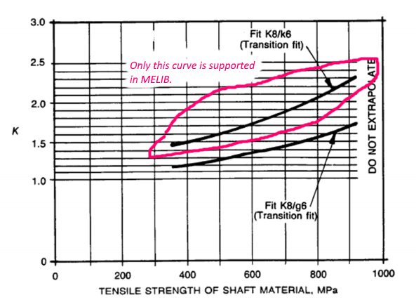
Calculates the stress concentration factor for a bearing seat with a K8/k6 transition fit according to AS1403 Figure 5. The other bearing fit in the AS1403 chart is not supported by this function.

The returned value is the stress concentration factor as per Figure 5 of AS1403.

Example

>>> bearingscf(800)
>>> 2.08896825088

melib.library.bmdiagram(P, p=0.5, L=1.0, Q=<Mock name='mock.zeros()' id='139896875537104'>, q=0, cc=[], draw=True, vlim=[], mlim=[], xlim=[], xcrit=[], yname='y', zname='z', filename='', fu='N', xu='m', record=False, debug=False)

This function can be used to draw the shear force and the bending moment diagrams and calculate the values of the bending moments in the nominated stress points and the reaction forces for a shaft represented as a simply supported beam supported by two bearings (B and C) and subject to two loads (P and Q) as in the following diagram:

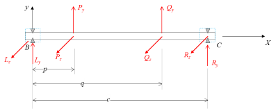
• P = [Py, Pz] in newtons

• p = Position of the P application point from the left end, m

• Q = [Qy, Qz] in newtons

• q = Position of the Q application point from the left end, m

• L = The distance between the two supports, m

You do not need to include q and Q if there is only one force. The other arguments are:

• draw : Will draw the shear force and bending moment diagrams if True

• xcrit : Will calculate the bending moments at these positions

• filename : Will store the diagrams in the image file “filename”.png

Examples

>>> P = np.array([-11280, 31000.0])
>>> Q = np.array([2860.0,   7860])
>>> p = 0.185
>>> q = 0.473
>>> L = 0.650
>>> xcrit = np.array([p, q])
>>> filename='examplebmdiagram'
>>> (M, B, C) = bmdiagram(P, p, L, Q, q, draw=True,xcrit=xcrit, filename=filename, record=True)

The above will create the following two image files:

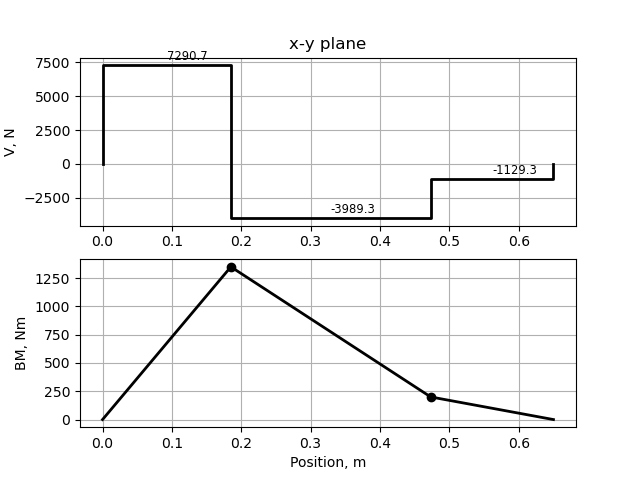
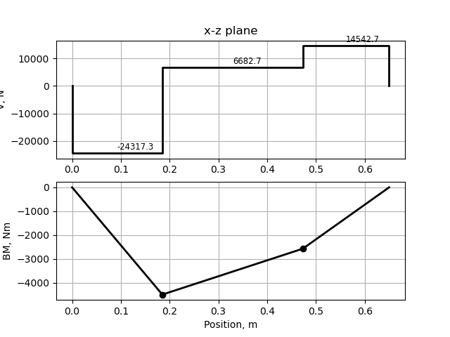
and will return

M = array ([[ 1348.8, 199.9], [-4498.7, -2574.1]])

B = array ([ 7290.7, -24317.3])

C = array ([ 1129.3, -14542.7])

melib.library.boltgrades(x, grade, props)

Arguments

x : Pointer to the bolts sheet in the materials data file

grade : Bolt grade, e.g. “4.8”

props : [“Dmin”,”Dmax”,”SUMPA”,”SYMPA”,”PROOF”] or a subset

Returns v

v[0] = Value from the file for ‘props[0]’

v[1] = Value from the file for ‘props[1]’

etc

Example

x=opendatafiles([“mats”])[0]

x.sheet(“bolts”)

v=boltgrades(xmat, “4.8”, [“Dmin”, “PROOF”])

print(v) # will print “[ 1.6 310. ]”

melib.library.boltpitch(dmajor, coarse=True)

Arguments

dmajor : Major diameter

coarse : True if coarse thread; False if fine thread

Returns pitch[mm] and stress area[mm2] as a tuple

Example

(pitch, At)=boltpitch(42, coarse=False) ==> pitch=3, At=1206

melib.library.density(metal, T=[])

Returns the density[kg/m3] of the metal. The optional second argument is the temperature[ ^o C]. Enter

>>> print(thconductivity("?"))

to see the supported metals.

melib.library.dgbbrtfacs(e=None, TC=None, Y=None)

This function is used in selection of a bearing subject to both radial and thrust loads. As you will see in the lectures, this is an iterative process and this function can be called repeatedly in search of a solution.

The function always returns a tuple with three components (e, TC, Y), one the same as the supplied value and the other two computed by the function. There are three arguments and only one should be specified.

e is specified. The function computes the values of T/Co and Y from the bearing thrust factors table (e.g. Mott Table 14-5)

TC (representing T/Co) is specified. The function computes e and Y

Y is specified. The function computes T/Co and e

Examples

>>> dgbbrtfacs(e=0.27)
>>> (0.27, 0.07, 1.63)
>>> dgbbrtfacs(TC=0.027)
>>> (0.218, 0.027, 2.01)
>>> dgbbrtfacs(Y=1.15)
>>> (0.38, 0.28, 1.15)

melib.library.ec3cutoff(detail)

Action

Eurocode 3 Cut-off limits for lattice girder joints as per Table 2.4 in Design Guide, Zhao et al

Argument

detail : The Detail category from Table B.2, e.g. 56 for K-joint with overlap

Return

Cut-off limit (the life is indefinite for stress ranges below this limit)

Example

>>> ec3cutoff(71)  # returns 32 MPa

melib.library.ec3life(nomstress, tr, joint='K', overlap=True, section='CHS')

Arguments

nomstress : Nominal stress range, MPa

tr : Wall thickness ratio (Chord thickness divided by brace thickness)

joint : ‘K’ or ‘N’

overlap : True if overlap joint; False if joint with a gap

section : Not used. Only CHS are supported

Returns N

N[0] = Life in cycles for the thickness ratio tr as given

N[1] = Life in cycles for tr as 1.0

N[2] = Life in cycles for tr as 1.40

Example

ec3life(120.0, 1.2, joint=’N’) # returns (80357,25866,134848) cycles

melib.library.fixity(econ, ideal=False)

Returns the value of the constant K in the Euler equation for buckling. The arguments are

econEnd conditions. Could be:

“pinned-pinned” “fixed-fixed” “fixed-free” (or “free-fixed”) “fixed-pinned” (or “pinned-fixed”)

idealReturns theoretical values if this True.

Otherwise, returns practical values

Example

>>> Ka=fixity("pinned-fixed")  # Actual value For pinned-fixed ends
>>> Ki=fixity("pinned-fixed", ideal=True)  # Ideal value For pinned-fixed ends

melib.library.geartip(dp, m)

Call with dp =pitch diameter and m =module both expressed using the same units , e.g. mm. The function returns the tip radius. It is assumed that the addendum is equal to the module.

Example : geartip(168, 8) –> 184

melib.library.huntingteeth(Np, Ng)

This function is used by the auto marker.

When the number of teeth on a pinion and the gear has common multiples, there may be preferential matching between gears and this would cause premature wear. When called with Np and Ng as the numbers of teeth on the pinion and the gear, respectively, this function returns

0 if Ng is an integer multiple of Np

0.5 if there is at least one common multiple, e.g. both are even numbers

1 if there are no common multiples

Examples

huntingteeth(23,46) –> 0

huntingteeth(22,46) –> 0.5

huntingteeth(23,47) –> 1

melib.library.isofits(X=None, d=60.0, s='H7f6')

Look up the upper and lower limits for the hole and the shaft for the specified fit. The only fits supported are

• Hxfy with x = 1,2,…,11 and y =3,4,…,9 and 3 < D <= 250

• Hxsy with x = 1,2,…,11 and y =3,4,…,9 and 3 < D <=1250

The data is read from the fits sheet in the shaft.xlsx file.

Examples

>>> isofits(d=60.0, s="H7f6")
>>> (30, 0, -30, -49)
>>> isofits(d=60.0, s="H7s6")
>>> (30, 0, 72, 53)
>>> isofits(d=110.0, s="H7s6")
>>> ((35, 0, 101, 79)
>>> isofits(d=2000.0, s="H7s6")
>>> SystemExit: isofits: nominal diameter (2000) is too large

melib.library.keyseatscf(uts, record=False)

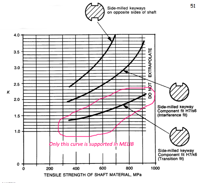
Calculates the stress concentration factor for a sidemilled keyway with a H7/k6 transition fit according to AS1403 Figure 7. The other keyways in the AS1403 chart are not supported by this function.

The returned value is the stress concentration factor as per Figure 7 of AS1403.

Example

>>> keyseatscf(650)
>>> 1.6365625047124999

melib.library.keysize(d)

Returns a tuple (width,height) for the specified diameter, d[mm] as per DIN6885, T1 (and also Table 11-1 in Mott).

Examples

>>> keysize(20)
>>> (6, 6)
>>> keysize(120)
>>> (32, 18)

melib.library.mintoothnum(phi)

Call with phi as the pressure angle in degrees. Returns the minimum number of teeth allowed on the pinion to prevent interference when driving a rack. The pressure angles of 14.5, 20, and 12 are supported. Reference is Mott, Table 8-7.

Example : mintoothnum(20) –> 18

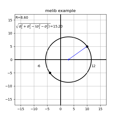
melib.library.mohrcircle(sx, sy, txy, filename='None', figno=1, title="2d Mohr's Circle")

For the 2d stress element:

This function returns the two principal stresses and the maximum shear stress as (s1, s2, taumax) in MPa.

The arguments sx, sy, txy are as in the figure.

If a filename is provided, the Mohr’s circle is drawn into that file.

Otherwise, it is drawn on the screen.

The figno and title are optional.

Example

>>> mohrcircle(10,-4,5,filename="mohrcircle.png", title="melib example")
>>> (11.60, -5.602, 8.602)

melib.library.opendatafiles(tags=['bearing', 'mats', 'sgear', 'shaft', 'vbelt'], makezip=False)

Action

Opens the Excel files in the data folder and returns file pointers.

Arguments

tags : Array of strings. Excel file names. All data files will be opened if tags is unspecified.

makezip : Boolean. Whether to add the files to a zip package (used in notebooks).

Returns

Xcel pointers to the data files. You may have to use these pointers when calling other library functions.

Example

>>> [Xbear, Xmat, Xgear, Xshaft, Xbelt]=opendatafiles()

melib.library.scf_roundbartension(D, d=10, r=1)

The stress concentration factor for a stepped round bar in tension

D, d, r are the dimensions as in the figure above in mm.

Example

>>> scf_roundbartension(200, 100, 10)
>>> 1.964

melib.library.scfa(k1, k2, k3=1, record=False)

Compute the combined stree concentration factors when two or three stress raising features coincide. The calculation is done as per AS1403 Article 8.2 (d) adapted to three features. The combined the SCF is the sum of the largest SCF plus 0.2 times the sum of the two lesser values. For example, if k2=max(k1,k2,k3) , then the returned value is k2+0.2*(k1+k3) .

Example

>>> scfa(2.0, 3.0, 4.0)
>>> 5.0

melib.library.shaftendur(uts, condition='ground')

Call with uts = Tensile strength[MPa] and condition = a string describing the surface condition. The returned value is the endurance strength read off the following chart: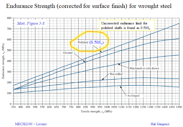

The valid options for the second argument are:

• 'ground' (default)

• 'polished'

• 'cold drawn'

• 'machined' (equivalent to 'cold drawn' )

• 'hot rolled'

Example

>>> shaftendur(900,'hot rolled')
>>> 212.5

melib.library.shaftreliability(rel)

rel is the desired target reliability, e.g. 0.10 for 10%

The returned value is the reliability factor CR

Example

>>> shaftreliability(0.99)
>>> 0.81

melib.library.shoulderscf(D, d, R, uts, record=False)

Calculates the stress concentration factor for a shaft shoulder according to AS1403.

D, d, R are the dimensions as shown in the figure above.

uts is the tensile strength in MPa.

The returned value is the stress concentration factor as per AS1403.

Example

>>> shoulderscf(200,100,10, 450)
>>> 1.6973600000014022

melib.library.shrinkscf(uts, record=False)

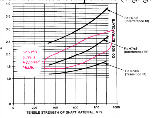
Calculates the stress concentration factor for a component fitted onto a shaft using a H7/s6 interference fit, according to Figure 6 of AS1403. The other two fits in the AS1403 chart are not supported by this function.

The returned value is the stress concentration factor as per Figure 6 of AS1403.

Example

>>> shrinkscf(400)
>>> 1.6204761921599997

melib.library.sizefactor(dia)

dia is the shaft diameter in mm

The returned value is the size factor CS read off a digitised version of the Mott chart Fig 5-9.

Example

>>> sizefactor(200)
>>> 0.6964150943396226

melib.library.steelprop(x, alloyname, props)

Short cut for alloyprop(x, “STEELS”, alloyname, props)

melib.library.thconductivity(metal, T=[])

Returns the thermal conductivity[W/m-C] of the metal. The second argument is the temperature[ ^o C]. Enter

>>> print(thconductivity("?"))

to see the supported metals.

melib.library.titanprop(x, alloyname, props)

Short cut for alloyprop(x, “titanium”, alloyname, props)

melib.library.unitconvert(fromunit, tounit)

Returns the coefficient to convert a number from one unit to another. For example,

>>> y=x*unitconvert("Calories_per_Cm2Min","W_per_M2")

will convert ‘x’ in units of ‘Cal/(cm2-min)’ to ‘y’ in ‘Watts/m2’.

The supported unit pairs are:

• “Calories_per_Cm2Min” —> “W_per_M2”

• “Grams_per_Dm2Hr” —> “Kg_per_M2H”

• “Lbf_inch” —> “N-m”

melib.library.vbeltc1(x, d, D, C)

Arguments

x : Xcel pointer to the belts data file

d : Diameter of the driving pulley[mm]

D : Diameter of the driven pulley[mm]

C : Centre distance[mm]

Returns

[1] = Wrap angle beta (for the driving sheave - see Optibelt catalogue p.73)

[2] = Arc contact correction factor c1 (Optibelt Catalogue Table 22)

Example

x=opendatafiles([“vbelt”])[0]

v=vbeltc1(x, 75, 230, 420)

print(v) # will print “(156.0, 0.99)”

melib.library.vbeltlengths(x, beltdes='5V', datumlength=673.0)

Arguments

x : Xcel pointer to the belts data file

beltdes : Belt designation, e.g. “3V” or “5V”

datumlength : Length target for the belt, mm

Returns values read from Optibelt Catalogue Table 25

[1] = Belt designation, e.g. “3V 1060”

[2] = Outside length[mm] of this belt designation

[3] = Length factor, c3

Example

x=opendatafiles([“vbelt”])[0]

v=vbeltlengths(x, “5V”, 673.0)

print(v) # will print “(‘5V 500’, 1270, 0.84)”

melib.library.vbeltpower(x, beltdes='5V', rpm=3000, dsheave=100.0, rat=2.0)

Arguments

x : Xcel pointer to the belts data file

beltdes : Belt designation, e.g. “3V” or “5V”

rpm : Speed of the driving pulley[rpm]

dsheave : Diameter of the driving pulley[mm]

rat : Speed reduction across this belt transmission stage

Returns values read from Optibelt Table 41(beltdes=3V) or 43(beltdes=5V)

[1] = PN(Nominal rating,kW) from Optibelt Catalogue Table 41(for 3V) or 43(for 5V)

[2] = Additional power per belt from Optibelt Catalogue Tables 41 or 43(3V or 5V)

Example

x=opendatafiles([“vbelt”])[0]

v=vbeltpower(x, “5V”, rpm=3000, dsheave=100.0, rat=2.0)

print(v) # will print “(24.98, 4.47)”

melib.library.weldsize(t)

Returns the minimum weld size[mm] for plate thickness ‘t’[mm]

Argument

t : Plate thickness in mm

Returns

The minimum weld size[mm] recommended for this plate thickness

Example:

weldsize(18.0) # returns 6.35 mm

Reference: Mott, Table 20-4 Minimum weld sizes for thick plates

xt.py

Routines to create markdown documents for Jupyter notebooks, PDF files, and some other useful stuff

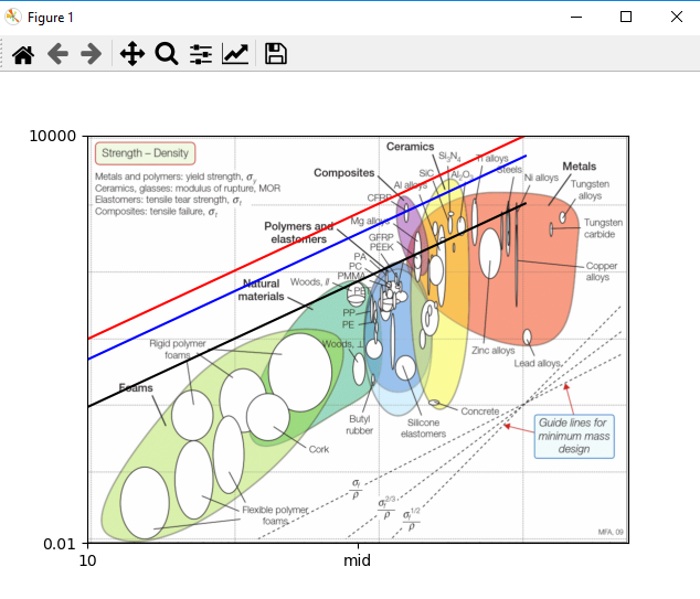
melib.xt.imgplot(X, Y, XXYY, cs='b-', imgfile='', ax=[], xticks=[], yticks=[])

This function is used to superimpose my curve on a chart image from a reference. The image should be the box only.

X , Y The data to be plotted (the same units as on the chart image)

XXYY The axis limits [[xmin, xmax], [ymin, ymax]] (from the reference image)

cs Plot line descriptor, e.g. "b--"

imgfile The name of the output, e.g. r"pics\Meshram_Fig6b.png"

ax This should not be included at first call. It is used to add curves later.

xticks x-axis tick positions you want to see, e.g. [“4000”, “midpoint”, “26000”]

yticks y-axis tick positions, e.g. [“ten”, “forty”, “seventy”, “hundred”]

The function returns (figno, ax). The ax can be used to add more y(x) curves:

e.g. imgplot(X2, Y2, XXYY, “r–”, ax=ax)

The XXYY in the second call should be the same as in the first

The ax in the second call is the same ‘ax’ returned by the first call

The figno can be used by the calling figure to save or to clear the figure

Example

>>> x = np.log10(np.arange(10, 10000, 100))
>>> y = x-np.log10(1.0)
>>> XXYY = [[1, np.log10(50000.0)], [-2, 4]]
>>> (f, ax) = imgplot(x, y, XXYY, cs='r-',imgfile=r"ashby_strength_density_chart_no_axes.png",xticks=[10, "mid", 100], yticks=[0.01, 10000])
>>> imgplot(x, x-np.log10(2.0), XXYY, 'b', ax=ax)
>>> imgplot(x, x-np.log10(10.0), XXYY, 'k', ax=ax)
>>> plt.show()

This example draws lines on the following reference chart:

To create the following plot:

class melib.xt.mdx(notebook, page=1, title='', initial='')

mdx is a pointer to a markdown file. I use it in creating lecture notes. A typical notebook have an iniialisation cell and then several chapter cells.

The structures for these cells are given below. Create a notebook named “XXXX.ipynb” and copy and paste the following code segments into that notebook as separate cells to create an example notebook generated using the mdx class.

Why should you use `` mdx `` ?

I found it clumsy to create markdown files with interactive live python code snippets in it when using standard markdown only.

Using the class mdx, all cells in the notebook can be code cells and the whole notebook can run as a single program.

The cell contents are created by using the mdx.write() method. There are special codes starting with ::: that can indicate headers, equations, insert images, and many other things. See the write-up for the write method.

Initialisation Cell

This will be the first cell in the ipynb file and it will have the following structure. This is initialisation for a notebook with three chapter cells and one reference cell at the end.

import math
import numpy as np
from IPython.display import Markdown as md
import matplotlib.pyplot as plt
import random
import sys
import os
from datetime import datetime, date
# import other packages as required
# ...
# ...
Chapter="XXXX"  # or any other name
YEAR=2021
TOC=["Chapter 1", "Chapter 2", "Chapter 3", "References"]
#
SECTION=0
MAKEZIP=True  # A zip file will be generated  (False otherwise)
#
# Module libraries
sys.path.insert(0,r"H:\My Documents\python")  # provide full path
sys.path.insert(0, r"H:\My Documents\melib_project\melib")  # provide full path
#
from xt import mdx, engfmt, mdxzipopen, mdzip, iswindows, openplot, plotanno
from excel import Xcel
LIBFILES=["xt.py", "library.py", "excel.py"]
#
if MAKEZIP: mdxzipopen(Chapter, LIBFILES)
#
MD=mdx(Chapter,0,title="Example Notebook")  # The markdown file pointer
MD.write("Created on 6 April 2021.   Last Update - "+date.today().strftime("%d/%m/%Y"))
MD.toc(TOC,"")  # Creates the table contents
MD.write("* The notebook source file is `%s.ipynb`"%Chapter)
#
md(MD.out())  # End of the initiation segment

The following is what you need to generate an HTML page from this notebook.

jupyter nbconvert XXXX.ipynb --no-input --to html

Chapter 1

This is the first chapter in the notebook following the initial cell. All contents will be inserted using the MD.write() function.

SECTION+=1
MD=mdx(Chapter, SECTION, TOC[SECTION-1])  # create the chapter file
MD.write("\n\n")
MD.write("... blah blah blah :::")
MD.write("... even more blah blah blah :::")
MD.write("\n\n")
md(MD.out())            # close the chapter file

Chapter 2

This is the second chapter in the notebook following the initial cell. All contents will be inserted using the MD.write() function.

SECTION+=1
MD=mdx(Chapter, SECTION, TOC[SECTION-1])  # create the chapter file
MD.write("\n\n")
MD.write("... blah blah blah :::")
MD.write("... even more blah blah blah :::")
MD.write("\n\n")
md(MD.out())            # close the chapter file

Chapter 3

This is the third chapter in the notebook following the initial cell. All contents will be inserted using the MD.write() function.

SECTION+=1
MD=mdx(Chapter, SECTION, TOC[SECTION-1])  # create the chapter file
MD.write("\n\n")
MD.write("... blah blah blah :::")
MD.write("... even more blah blah blah :::")
MD.write("\n\n")
md(MD.out())            # close the chapter file

One can have an arbitrary number of chapters. It is preferred to complete with one last segment on references:

The last content cell that contains the bibliography (optional)

SECTION=len(TOC)
MD=mdx(Chapter, SECTION, TOC[SECTION-1])
MD.write("Robert L. Mott, MECH2100 Machine Design (Custom Edition)\n\n")
MD.write("Ashby, M.F., 2011.   Materials selection in mechanical design, Butterworth-Heinemann, Oxford, OX ; Boston, MA .             (Electronic resource, Call Number:TA403.6 .A74 2011eb )\n\n")
MD.write("Standards Australia, 1993.  Engineering Drawing Handbook SAA HB7, Standards Association of Australia, (Call Number:T357 .M43 1993 )\n\n")
md(MD.out())

Read the following information on the `` write()`` method to see how you can generate cells with interesting content.

write(s)

This is the main method to populate the MDX notebook cells. Apart from the code segments, the string s is copied to the markdown file. The code segments start with ::: and end with ::

They are of the following format:

:::code|arg1|arg2::

where

code a number that defines the action

arg1 the first argument

arg2 the second argument

The following lists what is available through this construct:

:::2

:::2|HTML link|text:: The markdown document will display text that will link to the address defined in the first argument

Code 2 Example:

:::2|www.uq.edu.au|University of Queensland::

:::3

:::3|filename|caption:: will display the image in the first argument.

The image file is expected to be in the pics folder.

The figure numbers are automatically incremented. The second argument is optional. If omitted, then only the figure number will be shown:

Code 3 Examples

:::3|mohrcircle.png|Mohr's circle:: # with caption text :::3|mohrcircle.png:: # no caption

:::30

Similar to :::3 except that the image file is expected to be in the tmp folder.

:::32

Similar to :::3 except that the image file is expected to be in the ..\pics folder. This is useful when several notebooks use the same picture collection in the parent folder.

:::4

:::4|filename|cover text:: the cover text will be a link to a pop-up window

The image file is expected to be in the pics folder.

Code 4 Examples

:::4|mohrcircle.png|Click to see Mohr's circle:: # pop=up figure. The second argument is the cover text.

:::42

Similar to :::4 except that the image file is expected to be in the ..\pics folder. This is useful when several notebooks use the same picture collection in the parent folder.

:::5

:::5|equation|equation name:: The equation name can later be used to refer to this equation by number by using the eqnumber() function or :::6 command. The equation name may be left out.

Code 5 Examples

:::5|$sin^2(x)+cos^2(x)=1$|trig::

:::5|F=ma|Newton::

:::5|$y=x^2$::

melib.xt.mdxzipclose()

Do not use this function. It adds double back slash to the zip list file and it confuses zip file creation

melib.xt.mdxziplist(files)

It adds files to the zip listfile (see mdzip())

Args:

files (string array): Names of files to archive, e.g. [“xt.py”, “datmats.xlsx”]

melib.xt.mdxzipopen(notebook, libfiles)

Creates the zip file list and insert the ‘libfiles’ into it

Args:

notebook : Usually the name of the notebook but could be any string, e.g. “L20” libfiles : File names as an array of strings, e.g. [“xt.py”, “excel.py”]

The name of the list file will be notebook+”_zip.txt”

melib.xt.mdzip(zipfile, listfile)

Creates a zip archive of all components used in the notebook

Args:

zipfile : The name of the zip file to be created listfile : The text file containing the file names to be archived (optional)

For example,

mdzip(“L10”) – Will archive the list in “L10_zip.txt” into “L10.zip” mdzip(“xxxx”, “zzzz.txt”) – Will archive the list in “zzzz.txt” into “xxxx.zip”

melib.xt.openplot(figno, aspect=[])

Arguments

figno : Figure numbers

aspect : Aspect ratio, e.g. 0.5 for a rectangle width=2*height

Returns (f1, ax)

f1 = Pointer to the figure (can be used to save the figure, e.g. f1.savefig(“myfigure.png”)

ax = Pointer to the plot axes (use this to plot, e.g. ax.plot((x, y, “r”, label=”Y”)))

Example

>>> x=np.arange(0,10,0.01)
>>> y=np.sin(x)
>>> (f1,ax)=openplot(1,0.5)
>>> ax.plot(x,y,"m",label="sine")
>>> plotanno(ax,xlabel="X variable", ylabel="sin(x)", xlim=[1,9], ylim=[0, 1.0], grid="on", legendloc="upper right", title="Example - y=sin(x)")

melib.xt.plotanno(ax, xlabel='', ylabel='', xlim=[], ylim=[], grid='on', legendloc='', title='')

For the matplotlib figure axis pointer ax:

Add axis labels (xlabel and ylabel ) Axis limits, e.g. xlim (=``[xmin, xmax]`` ) Location for the legend , eg “upper right” Turn the grid lines on and off and a figure title

Example

>>> x=np.arange(0,10,0.01)
>>> y=np.sin(x)
>>> (f1,ax)=openplot(1,0.5)
>>> ax.plot(x,y,"m",label="sine")
>>> plotanno(ax,xlabel="X variable", ylabel="sin(x)", xlim=[1,9], ylim=[0, 1.0], grid="on", legendloc="upper right", title="Example - y=sin(x)")

excel.py

Methods that are used in melib to read, edit and generate excel files

The data folder has design data that are needed by the functions in the library.py file.